Hiding a message in the noise of a camera
How natural steganography hides data in JPEG photographs by adding the noise of a higher ISO: from the sensor through demosaicking to the DCT, the dependencies that creates, and how to draw a signal that respects them.
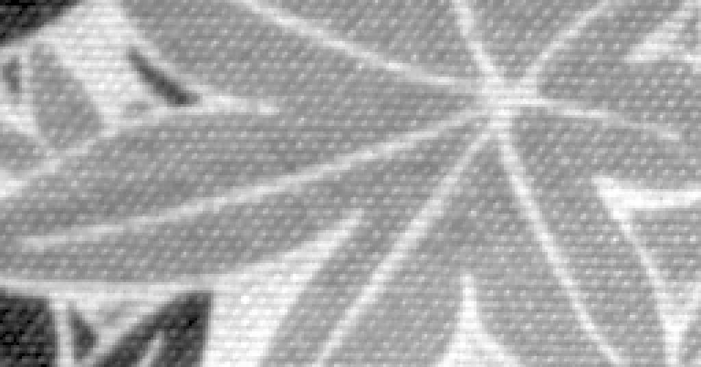
Two photographs of the same piece of cloth. One was taken at ISO 200. The other was taken at ISO 100, then given the noise it lacked to pass for ISO 200, drawn so that it could carry a payload. Can you tell which?
The crop that could carry a payload is the work of natural steganography: a message is hidden not in changes too small to see, but in a whole layer of noise that the camera could have made itself. This article explains the scheme my co-authors and I published in IEEE TIFS[1], J-Cov-NS, from the sensor to the JPEG file.
One number runs through it: how much a picture can carry. In the paper’s tests, SI-UNIWARD, a classic JPEG scheme, is caught every time at QF 100 with one bit per non-zero AC coefficient. J-Cov-NS carries two on average, and the same detector errs 43 % of the time, where a coin toss would err 50 %. Getting there means following the noise through demosaicking and the DCT, finding the dependencies that creates, and drawing a signal that respects them.
Most figures compute what they show, in your browser, from the paper’s maths and two of its RAW files; the last one charts the paper’s own tables. The embedding is simulated, as in the paper: the bits are counted, not written.
The sensor’s noise is a budget
A camera sensor counts photons, and the count is noisy. This photonic noise is Gaussian to a very good approximation, and its variance grows with the light: $\sigma^2 = a\,\mu + b$, where $\mu$ is the noiseless value of the photosite. Raise the ISO and the sensor amplifies harder, so the same scene shot at ISO 200 is noisier than at ISO 100.
Natural steganography[2] lives in that gap. Starting from an ISO 100 picture $x$, it adds at every photosite a stego signal
\[S \sim \mathcal{N}\big(0,\ (a_2 - a_1)\,x + b_2 - b_1\big),\]so that the result is distributed as an ISO 200 shot of the same scene would be: equal in distribution, in the paper’s words (eq. 8), as long as the photosite’s value is close to its expectation.1 Nothing is hidden by keeping the changes small. A whole layer of noise is added, and it is allowed to be there: the only limit on how much it can carry is the gap between the two ISOs.
From photosites to JPEG coefficients
The stego signal is added where the noise lives, on the photosites, before the camera has done anything with them. The message, though, travels in a JPEG file, and between the two lies the whole development of the picture. Follow the noise of a single photosite through it.
A sensor does not see colour. Each photosite sits under a red, a green or a blue filter, laid out in the Bayer pattern. Here is a patch of 26×26 of them, and one red photosite carrying a burst of noise. Every other photosite is left alone, so what follows is the trace of that one value. Any other photosite of the dashed square, the centre block, can take its place, but the text follows the red one.
Demosaicking fills in, at every pixel, the two colours its photosite did not measure. With bilinear interpolation, the red of a pixel is a weighted average of the red photosites around it: 1 for its own, ½ for a side neighbour, ¼ for a diagonal one. The burst now shows in nine pixels. This is $D$.
The paper works on greyscale JPEGs, which keep one plane, the luminance $Y = 0.299\,R + 0.587\,G + 0.114\,B$. The burst only touched red, so it reaches $Y$ at 0.299 of its strength, still over nine pixels. This is $L$.
JPEG cuts the picture into 8×8 blocks. The photosite sat at the edge of one: its nine pixels straddle two blocks, the centre one, C, and its east neighbour, E. The rim of photosites around the blocks is there because demosaicking reads one photosite past them. $S$ selects the pixels of the blocks, $P$ puts them in block order.
Each block goes through an 8×8 DCT, $T$: 64 coefficients, one per frequency, the low ones top left. One photosite now moves all 64 coefficients of both blocks at once, with fixed signs and proportions. That is one column of $M = T\,P\,S\,L\,D$, the linear map from photosites to DCT coefficients. Noise that was independent from one photosite to the next comes out correlated: within a block, and across the border between blocks.
Last, each coefficient is divided by its step in the quantisation table of the chosen quality, and rounded to the integer the file stores. For anything to survive here, the burst is 1,500 DN, about ten times the noise of a bright photosite at ISO 200. Lower the quality and the steps grow: fewer coefficients survive. Natural steganography draws these integers, which is why it carries the most at high qualities.
The DCT step is worth a closer look, because a DCT coefficient is not a pixel: it measures a pattern. Each of a block’s 64 coefficients belongs to one of the 64 patterns below, products of two cosines, one across the block and one down it, slow at the top left and fast at the bottom right. The coefficient is how much of its pattern the block holds: the block and the pattern multiplied pixel by pixel, then summed. The patterns are orthogonal, so the block is also the sum of its 64 patterns, each weighted by its coefficient: that is the inverse DCT.
The burst sits on the right edge of C and the left edge of E, and every pattern has something there, so every pattern picks it up. That is why the red photosite moves all 128 coefficients of its two blocks, with signs and proportions that the patterns alone decide, whatever the photosite’s value. Pattern (0, 1), half a cosine across the block, is positive on the left and negative on the right: it meets the burst on its negative side in C and on its positive side in E, and the two coefficients come out with opposite signs. The quantisation table of the last step is laid out the same way, one step per pattern, coarse for the fast ones.
Other photosites tell the same story with other numbers. A green one counts for 0.587 of the luminance, but its kernel is a cross of five pixels, so at a block’s corner it reaches three blocks and never the diagonal one. A blue one counts for 0.114, and at QF 85 one of its coefficients survives rounding at most. A photosite in the middle of a block stays in that block.
That was one photosite. A real stego signal puts its own noise on every photosite at once, each independent of the others, and each leaves its own column of $M$ in the DCT domain. Their sum is a field of noise whose coefficients are tied together: within a block, because a block is made of the same photosites, and across blocks, because demosaicking reads one photosite past each block’s edge.
Why neighbouring blocks move together
The development is linear, so the noise it leaves in the DCT domain is Gaussian too, with a covariance the paper writes in closed form (eq. 24):
\[\Sigma = M\,\mathrm{diag}(v)\,M^\top,\]where $v$ is the variance of the stego signal at each photosite. The photosites are independent of each other. The coefficients are not: neighbouring pixels share photosites through demosaicking, and the 8×8 blocks of a JPEG sit side by side on the same sensor.
Pick a coefficient of the centre block. It moves most with the other coefficients of its own block, less but clearly with the four blocks that share a side with it, and hardly at all with the four diagonal ones, which only meet it at a corner. The three developments take this apart, as Fig. 8 of the paper does inside one block. With the red channel alone, the Bayer pattern shows through: the red photosites sit in the north-east corner of each 2×2 cell, so a block no longer depends on its four sides alike. For the low frequencies, (0, 1) among them, the dependencies lean towards north and east; for the highest, towards south and west. With the paper’s plain low-pass filter and no mosaic, opposite sides mirror each other again.
The middle picture is all of $\Sigma$ at once, as correlations: a row and a column per coefficient, 64 for each block, in the order C, N, W, E, S, then the corners. Each of its 9×9 squares is a pair of blocks. On the diagonal, each block with itself, the brightest, up to 0.84. Fainter, two blocks that share a side, up to 0.11. Near black, two that meet only at a corner, under 0.01, or not at all, like N and S. The outlined row is the chosen coefficient’s: the picture on the left is that row, laid back out as blocks.
The picture on the right says why. It is the chosen coefficient’s column of $\Sigma$ put back through the inverse DCT: what knowing that one coefficient tells about each pixel around. Inside its block, its own DCT pattern. Past each side, a trace one or two pixels deep, where the neighbouring block was demosaicked from the same photosites as the edge of this one. Nothing reaches the diagonal blocks but a corner.
Why drawing each coefficient on its own fails
Knowing $\Sigma$, the tempting shortcut is to keep only its diagonal: draw each coefficient on its own, with the right variance, as the first JPEG version of natural steganography did[3]. Every coefficient then has exactly the right histogram, and on a monochrome sensor, where nothing ties neighbouring pixels together, that is enough. On a colour sensor it is not.
Back in pixels, the eye can hardly tell them apart. The numbers can. Inside a block, neighbouring pixels move together about as much in both draws. That hides a loss there too: the coefficients of one block are tied to each other, (0, 7) and (7, 0) at a correlation of 0.84, through the Bayer pattern, and the independent draw cuts those ties as well. Across a block border, the independent draw has nothing tying the two sides together, and the correlation drops to zero. The joint draw runs on across the border, like the noise of a real sensor.
A detector that looks at the picture relative to the 8×8 grid, as phase-aware features such as DCTR[4] do, sees this at once. The paper measures it with $P_E$, the detector’s error at its best threshold, from 0 % (always caught) to 50 % (a coin toss). Drawn independently, coefficient by coefficient, the signal is caught every time at QF 100, $P_E = 0.0\,\%$. Drawing each block’s 64 coefficients jointly but the blocks independently of each other does no better. J-Cov-NS, which ties the blocks together, stays at 42.9 %.
Four lattices of blocks
Drawing a whole photograph at once would take a covariance with as many rows as the picture has coefficients: millions. The paper draws one block at a time instead, given the neighbours already drawn, and only the eight that touch it: past them, as the previous figures showed, nothing is shared. The order matters, and the paper settles it with four interleaved lattices, Λ1, Λ2, Λ3 and Λ4, drawn one after the other. That is the chain rule:
\[p(\Lambda_1, \Lambda_2, \Lambda_3, \Lambda_4) = p(\Lambda_1)\; p(\Lambda_2 \mid \Lambda_1)\; p(\Lambda_3 \mid \Lambda_1, \Lambda_2)\; p(\Lambda_4 \mid \Lambda_1, \Lambda_2, \Lambda_3).\]Here are 12 by 8 blocks, nothing drawn yet. Each block will be drawn given the blocks around it that are already drawn, and only those.
Λ1 first: every other block on every other row. No two of them touch, not even at a corner, so each is drawn on its own law, given nothing. A quarter of the picture, all at once.
Λ2 next, the blocks diagonally between them. Each meets four Λ1 blocks at its corners, already drawn, and is drawn given those. Corners share few photosites, so it loses little.
Λ3 fills the gaps along the rows. Its four sides, two Λ1 blocks and two Λ2 blocks, are all drawn, and a side is a strip of photosites two wide that both blocks read, twenty of them, where a corner shares four: its law narrows, and it carries a quarter less.
Λ4, the last quarter, is surrounded. All eight of its neighbours are known, and it is drawn given them all, with the narrowest law and the fewest bits. Turn on the reach to see how far back a single Λ4 block depends.
The figure’s bits per block come from a flat, bright patch (6000 DN), where the noise is strong. The paper’s Fig. 14, on a synthetic flat image, gives about 0.8 bit per pixel for Λ1 down to 0.4 for Λ4 at QF 100: the same order, with a steeper fall: half from Λ1 to Λ4 there, about a third here.
The draw, in miniature
Before a real block of 64 coefficients, two. They show the whole routine at a size that fits on a page.
Take two DCT coefficients whose noise moves together, with a correlation $\rho$. Their joint law is a Gaussian, drawn here as an ellipse. The grid is the JPEG quantisation: one square for each pair of integers the file can store.
The first coefficient is drawn from its own law. Quantised, that law becomes a handful of probabilities, one per integer: the PMF of eq. (29).2 An integer is picked from it. Then a continuous value that rounds to that integer is found again by rejection: draw from the Gaussian, keep the first value that lands in the right square.
The second is drawn knowing the first. Its law is still Gaussian, but slid to $\rho\,s_1$ and narrowed to $\sqrt{1-\rho^2}$: the Schur complement, at the size of a $2\times2$ matrix. Same routine: PMF, integer, rejection.
Do it a thousand times and the draws fill the ellipse, as photonic noise would. Drawn each on its own, with the very same histograms, they fill a round cloud instead. That difference is what a steganalyser learns to see.
The real scheme writes the same thing as $s = m + L\,n$: a vector $n$ of independent standard normals, bent into shape by $L$, the Cholesky factor of the covariance. Here $L$ is $2\times2$. For a real block it is $64\times64$, worked out after conditioning on up to eight neighbouring blocks.
Conditioning has a price. Once the first coefficient is known, the second is less uncertain, so it carries fewer bits. The stronger the correlation, the more the scheme gives up, which is why the capacity falls from one lattice to the next.
Drawing one real block
Back to the two coefficients of the miniature, now at full size: a block of 64, given its eight neighbours. The routine is the same; only the matrices grow.
Conditioning happens in the DCT domain. Here are a Λ4 block and its eight neighbours, 64 coefficients each, laid out as the blocks lie. The neighbours are drawn already, each coefficient coloured by its value over its own $\sigma$. The centre is not drawn yet, but it is no longer unknown either. Given the neighbours’ coefficients $x_n$, its own have a Gaussian law whose mean is a weighted sum of theirs, $\mu = \Sigma_{cn}\,\Sigma_{nn}^{-1}\,x_n$, and the centre fills in with it. A new draw of the neighbours gives it another.
Its spread narrows too, to $\Sigma_{cc} - \Sigma_{cn}\,\Sigma_{nn}^{-1}\,\Sigma_{nc}$, the Schur complement. Here is each centre coefficient’s $\sigma$ given the neighbours over its $\sigma$ alone. The low frequencies learn the most: at (1, 1), $\sigma$ falls to 0.66. The high ones keep about 0.9. In all, the neighbours account for a third of the block’s variance, and what they already say, the block can no longer carry.
Now the centre block alone, and one coefficient up close: its law against the integers the file can store, each bin one quantisation step wide. The block is coloured by that law’s $\sigma$ over the step. At QF 100 the low frequencies spread over several integers: (0, 1) has $\sigma$ = 0.79 steps. The high ones, which demosaicking smooths away, fit inside one: (7, 7) has 0.04. Hover or tap them to compare.
The block is drawn coefficient by coefficient, row by row, each given the neighbours and the coefficients already drawn, and it fills in with the integers drawn. Up close, the coefficient’s PMF over the integers, the one picked in red, then a value inside that bin found by rejection: the ticks under the axis, misses faint.
Each coefficient drawn tells something about the ones after it, so their laws narrow as the block fills in. The block shows by how much: the first four rows by about a fifth, the last four, drawn after nearly all the others, by 60 to 80 %. Up close, dashed, the law given the neighbours only; solid, given the coefficients before it too. Pick (4, 0): $\sigma$ falls from 0.65 of a step to 0.21.
What a coefficient carries is the entropy of its PMF, and the block’s capacity is their sum, as in the paper’s Fig. 14. Switch to QF 95: the high frequencies get steps up to 12 times wider, their laws fit in a single integer, and their bits are gone.
How much it carries
The paper measures security as the field does. It trains a detector to tell apart 5,400 pairs of equivalent scenes, one shot at ISO 200, the other shot at ISO 100 and given the stego signal. Then it reports the detector’s error, $P_E$, on 5,400 more pairs. At 50 %, the detector is guessing.
At QF 100, J-Cov-NS has room for 2 bits per non-zero AC coefficient on average, and the detector is wrong 42.9 % of the time: barely better than a coin toss. In the same test, SI-UNIWARD[5], a classic adaptive scheme that hides by changing as little as it can, is caught every time with half that payload.
The other points are other ways of drawing the stego signal, all from the paper’s Table I. Pseudo-embedding adds the noise on the photosites and develops the result, as a camera would. It carries no message, but it is the reference for what the noise should look like, and J-Cov-NS matches it. Covariance scaling, our earlier scheme[6], estimated $\Sigma$ once on a flat picture and scaled it by each block’s average colour: good enough at QF 85 and 75, caught far more often at 100 and 95. Coefficients drawn independently, from histograms learnt mode by mode[3], and blocks drawn independently with their inner correlations kept, are both caught every time at QF 100. Against SRNet[7], a deep detector, J-Cov-NS still keeps 31 to 37 %.
In bits per pixel, J-Cov-NS carries about 0.45 at QF 100 and 0.2 at QF 95 on E1Base (the paper’s Fig. 13a, read off the plot): some 15 KB in a 512×512 picture at QF 100, and 6.5 KB at QF 95. The crop at the top of this page could carry almost 6 KB in 256×256 pixels, more per pixel than E1Base’s average. At the crop’s rate, 0.7 bit per pixel, a 16-megapixel photograph would carry over a megabyte; that is an extrapolation, not a measurement.
The alphabet has to be wide enough as well. Each coefficient is drawn among the $2K+1$ integers around the centre of its law; with $K = 1$, too few to follow the tails of the Gaussian, the detector catches J-Cov-NS at QF 100 99 times out of 100. With $K = 5$ it is back to 40 %.
Limits
None of this comes free.
- It needs the RAW. The stego signal lives on the photosites, so the sender must hold the RAW file, know the sensor’s noise at both ISOs, and develop the picture with a known pipeline: here, as in the paper, bilinear demosaicking and a greyscale JPEG.
- It is slow. Each block needs its own conditional law and its own Cholesky factor: 171 s for a 512×512 picture in the paper, with Λ4 blocks drawn at 10 a second.
- The alphabet must be wide. This page draws each coefficient among 11 integers ($K = 5$); with 3, the scheme is caught at QF 100.
- Deep detectors do better. SRNet brings $P_E$ down to 31–37 %: far from caught, no longer a coin toss.
- The embedding is simulated. Here, as in the paper’s experiments, the capacity is the sum of the entropies of the PMFs, and the draws are what a perfect code would produce. A real message would be written with multi-layered syndrome-trellis codes[8], which come close to that bound, with costs derived from the same probabilities.
Going further
The paper[1] has what this article leaves out: the full construction of $M$, the derivation of the conditional laws, and more experiments. Around it, other pieces of the same work: an empirical study of colour JPEG steganography and steganalysis[9]; the computation of dependencies between DCT coefficients[10], which this scheme builds on; the synchronisation of DCT coefficients for a given development pipeline[11], the same idea for adaptive schemes; and the thesis that gathers them[12], in French. The reference code and notebooks[13] accompany the paper, and E1Base holds the 10,800 crops of its experiments, cut from 200 RAW photographs; the links are in the appendix.
Acknowledgements
From the paper: the authors thank Solène Bernard (CRIStAL, Lille) for running the experiments with SRNet. The work was granted access to the HPC resources of IDRIS under the allocation 2020-AP010611583 made by GENCI, and to those of the University of Lille. It was funded in part by the French National Research Agency, through the ALASKA project (ANR-18-ASTR-0009) and the DEFALS program (ANR-16-DEFA-0003).
This page draws its figures in your browser with D3 and GSAP, from the RAW files and the reference code that come with the paper. Its layout owes everything to Distill.
References
- T. Taburet, P. Bas, W. Sawaya, J. Fridrich. Natural Steganography in JPEG Domain With a Linear Development Pipeline. IEEE Transactions on Information Forensics and Security, vol. 16, pp. 173–186, 2020.
- P. Bas. Steganography via Cover-Source Switching. IEEE International Workshop on Information Forensics and Security (WIFS), 2016.
- T. Denemark, P. Bas, J. Fridrich. Natural Steganography in JPEG Compressed Images. Electronic Imaging, Media Watermarking, Security, and Forensics, 2018.
- V. Holub, J. Fridrich. Low-Complexity Features for JPEG Steganalysis Using Undecimated DCT. IEEE Transactions on Information Forensics and Security, vol. 10, no. 2, pp. 219–228, 2015.
- V. Holub, J. Fridrich, T. Denemark. Universal Distortion Function for Steganography in an Arbitrary Domain. EURASIP Journal on Information Security, vol. 2014, no. 1, 2014.
- T. Taburet, P. Bas, W. Sawaya, J. Fridrich. A Natural Steganography Embedding Scheme Dedicated to Color Sensors in the JPEG Domain. Electronic Imaging, Media Watermarking, Security, and Forensics, 2019.
- M. Boroumand, M. Chen, J. Fridrich. Deep Residual Network for Steganalysis of Digital Images. IEEE Transactions on Information Forensics and Security, vol. 14, no. 5, pp. 1181–1193, 2019.
- T. Filler, J. Judas, J. Fridrich. Minimizing Additive Distortion in Steganography Using Syndrome-Trellis Codes. IEEE Transactions on Information Forensics and Security, vol. 6, no. 3, pp. 920–935, 2011.
- T. Taburet, L. Filstroff, P. Bas, W. Sawaya. An Empirical Study of Steganography and Steganalysis of Color Images in the JPEG Domain. International Workshop on Digital Watermarking (IWDW), Springer, 2018.
- T. Taburet, P. Bas, J. Fridrich, W. Sawaya. Computing Dependencies between DCT Coefficients for Natural Steganography in JPEG Domain. ACM Workshop on Information Hiding and Multimedia Security, pp. 57–62, 2019.
- T. Taburet, P. Bas, W. Sawaya, R. Cogranne. JPEG Steganography and Synchronization of DCT Coefficients for a Given Development Pipeline. ACM Workshop on Information Hiding and Multimedia Security, pp. 139–149, 2020.
- T. Taburet. Méthodes de stéganographie fondées sur la prise en compte du bruit de capteur. PhD thesis, École Centrale de Lille, 2020.
- T. Taburet, W. Sawaya, P. Bas, J. Fridrich. Python Implementation of Natural Steganography: Notebooks Accompanying the Paper Published in IEEE TIFS. Software, 2024.
Cite this work
The paper this article explains:
@article{taburet2020natural,
  author  = {Taburet, Th{\'e}o and Bas, Patrick and Sawaya, Wadih and Fridrich, Jessica},
  title   = {Natural Steganography in {JPEG} Domain With a Linear Development Pipeline},
  journal = {IEEE Transactions on Information Forensics and Security},
  volume  = {16},
  pages   = {173--186},
  year    = {2020},
  doi     = {10.1109/TIFS.2020.3007354}
}Code and data
- The paper, open access: HAL hal-02910206, and on IEEE Xplore.
- The reference code, notebooks and the two RAW files these figures start from: tifs-ns, also archived as HAL hal-04456456.
- E1Base, the database of the experiments, 10,800 crops of 512×512 cut from 200 RAW photographs at ISO 100 and 200: e1base.
- The code of this page and its tests: assets/js/ns, with the maths checked against the reference code in tools/ns-check.mjs.
Where $(a_2 - a_1)\,x + b_2 - b_1$ would be negative, in the darkest parts of the picture, the paper sets the variance to 0: nothing is added there, and nothing can be carried. ↩︎
Eq. (29) centres these probabilities on the stego signal’s mean alone, as if the cover’s coefficient sat on a quantisation step. This page centres them on the cover’s coefficient plus that mean: the law of the integer the file stores, which is also what the paper’s code gets by rounding the cover plus the signal. Where the cover’s coefficient falls between two steps, that integer is less certain, and carries more: on the crop at the top of this page, 4.5 % more bits at QF 100 and 20 % more at QF 95. ↩︎